Phase 6 — Tool Loops, Termination, and What the User Actually Feels

The response has finished streaming. The chat bubble shows the assistant’s reply. The composer is unlocked. From the user’s perspective, the request is over.

From the serving stack’s perspective, three things still might be in flight. There is a tool call the model emitted that needs to execute and feed back through Phase 2 through 5 all over again. There is final billing accounting that has to settle. There is a latency story that explains why the request felt the way it felt, which is most of what the user actually noticed.

The tool loop

When the model emits a tool call instead of a final answer, the request is not done. The agentic loop has just started.

The model’s output (or a structured portion of it) is a function call: a tool name and a JSON-shaped argument blob. The serving stack parses the call out of the stream, halts further generation, and hands control back to the developer’s code. The developer’s code runs the requested tool (a local function, a database query, a web search, a code execution sandbox, an MCP server call) and produces a result. The result is formatted as a new message in the conversation, typically with role tool or its vendor-specific equivalent, and the augmented conversation is fed back into the model.

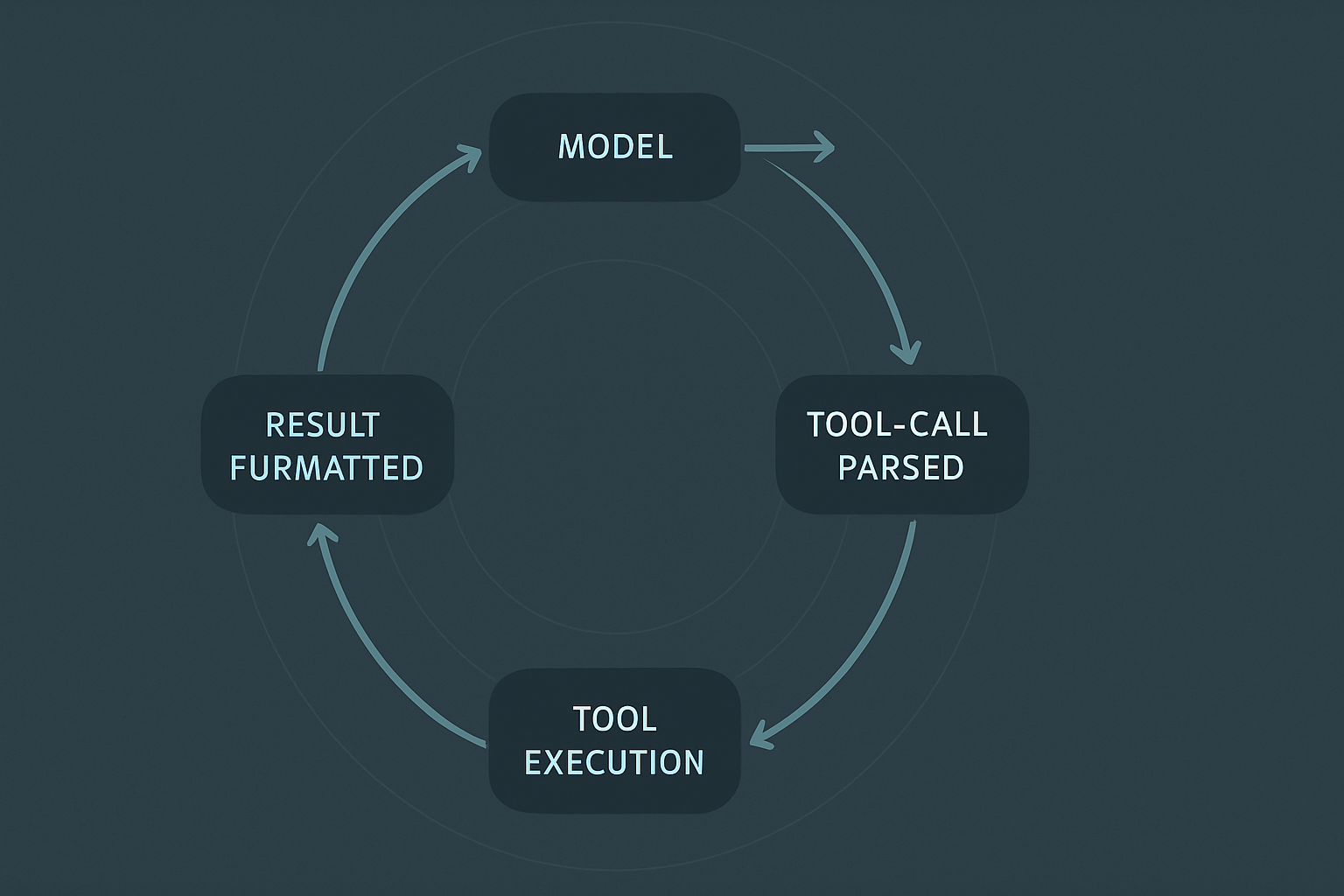
The augmented conversation triggers a new prefill. Phase 3 begins again. The model sees its own prior tool call, the tool’s result, and everything that came before, and it produces the next output. That output might be another tool call (loop again), or a final answer for the user, or in some agent designs, a planning step that leads to several tool calls in sequence.

A few mechanics matter for the developer.

The conversation grows monotonically. Every loop adds at least two messages: the assistant’s tool call and the tool’s response. Long-running agents accumulate context faster than most developers expect. A multi-step agent that runs ten loops on a 4,000-token initial prompt with 500-token tool responses ends up running its final prefill against 9,000+ tokens. Prompt caching across loops is what keeps this affordable. Without it, every loop pays the full prefill cost of the entire accumulated context.

Tool results are not validated by the model side. The serving stack does not check that a tool’s response is well-formed JSON, that it matches a schema the model expected, or that the content is safe. The developer’s code does. A tool result that is malformed gets fed to the model as-is, and the model attempts to recover by producing another tool call or by guessing. The recovery quality is uneven. Production agent stacks typically wrap tool results in their own validation layer.

MCP has changed the landscape. Model Context Protocol, formalized by Anthropic in late 2024 and adopted across vendors through 2025, gives tools a standard runtime interface that any model can call. An MCP server exposes a set of tool definitions over a standard transport (typically stdio or HTTP), and any MCP-aware client (Claude Desktop, Cursor, Continue, the OpenAI Agents SDK, the various agent frameworks) can use them without per-tool integration code. In 2026 most production tool integration goes through MCP rather than per-model function-calling adapters.

Loop limits matter. Without a maximum-iterations cap, a confused agent can loop forever, calling tools in an endless cycle of attempted recoveries. Every production agent framework enforces a max-loops setting. Most default to 10 or 20 iterations. The right number depends on the task; the principle is that you cap it explicitly rather than letting the loop run unbounded.

Streaming complicates everything. When the model is generating with streaming enabled, the gateway has to detect mid-stream that the output is a tool call rather than text, halt the stream, parse the partial-but-complete tool-call delta, and hand control to the developer. Different vendors expose this differently. Phase 5 covered the chunk-level mechanics. The developer’s framework code typically hides the complexity behind a single event handler.

Deeper: why “agentic” is mostly the same loop you have already seen.
The agentic AI category, which has dominated mid-2020s discourse, is structurally just this: Phase 3 through Phase 5, in a loop, with the loop body deciding which tool to call next and the loop termination decided by the model itself. There is no separate “agent inference” mechanism. The model runs the same prefill-decode-stream cycle it would run on a single-turn request, and the only difference is that the conversation context grows each loop. The interesting engineering questions in production agents are about loop control, context compression, tool result validation, and cost management of long contexts. None of those are fundamentally inference questions. They are wrapper questions of the kind covered in Phase 1 and Phase 2.

When the model finally returns a tool-free answer, the loop exits. The streaming finishes through Phase 5 as a normal response. The request moves into termination.

Termination and the receipt

The request closes. Several things have to settle before the connection goes back to the pool.

Final usage accounting and billing. This is the receipt. Token usage is not one number. Modern hosted APIs price four classes of tokens separately, and a serious developer reads all four.

Input tokens are the prompt and conversation history (and tool definitions, for tool-using requests). Priced at one rate.

Output tokens are the tokens the model generated. Priced at a higher rate, typically two to five times the input rate, because output tokens cost more to produce: decode is sequential while prefill is parallel.

Cached input tokens are input tokens served from a prompt cache hit. Priced lower than fresh input tokens, typically 10% to 50% of the regular input rate, because the vendor avoided most of the prefill compute. The savings are real and add up fast on stable system prompts.

Reasoning tokens are the hidden thinking-channel output of reasoning-mode models (the o-series, DeepSeek-R1, Claude extended thinking, Gemini thinking). They are counted toward output cost and the developer pays for them even though the user never sees them. On a long-reasoning request, reasoning tokens can dwarf the visible-answer tokens by a factor of 10 or more.

A request that issued a tool call has accounting from each loop. The billing commit aggregates all of them. The trace context preserves the breakdown by loop iteration, which is what makes per-step cost attribution possible after the fact.

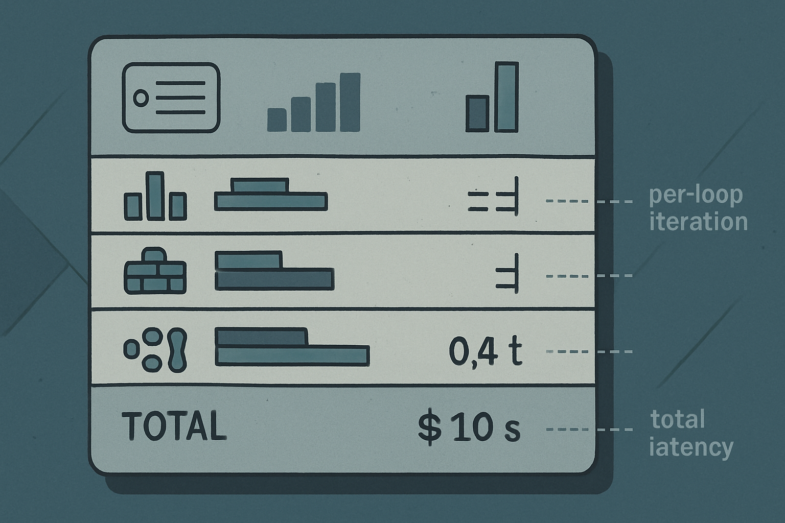
Prompt-cache write. If the request added new cacheable prefixes (a fresh system prompt that future requests will share, a long context document the developer flagged with cache control), the gateway writes the resulting KV cache blocks to the prompt-cache memory pool. The next request that hits the same prefix will pay the cache-hit rate instead of the full prefill cost. The write itself is asynchronous and doesn’t block the response.

Observability close. The trace span opened at admission is closed. Final metrics emit: tokens by class, latency by phase (TTFT, total decode time, tool-loop time if any), HTTP status, model version routed to, prompt-cache hit ratio. Eval sampling fires (some requests get duplicated to evaluation pipelines for ongoing model-quality monitoring). Safety telemetry posts to the moderation review queue.

Connection cleanup. The HTTP connection returns to the keep-alive pool for the next request from the same client, or closes if the client requested Connection: close. The KV cache for this specific request is freed and its blocks return to the pool for the next sequence.

The request is now formally done. The numbers are committed. The bill is final. From the developer’s perspective, everything is observable, billable, and gone.

The latency model: what the user actually feels

Two numbers describe the latency profile of an LLM request. Every other latency metric on a serving dashboard is a derivative of these two.

Time to First Token (TTFT). The interval from when the request hit the gateway to when the first output token arrives at the client. TTFT is dominated by prefill plus any queueing time before prefill started, plus the network round trip for the first chunk. It is the “spinner” interval that users perceive as “the model is thinking.” A TTFT under one second feels responsive. A TTFT of three to five seconds feels slow. A TTFT above ten seconds feels broken regardless of how good the response eventually is.

Time per Output Token (TPOT), also called Inter-Token Latency (ITL). The average interval between successive output tokens once streaming has started. TPOT is dominated by decode, which is memory-bandwidth-bound on every modern serving stack. A TPOT of 30 to 50 ms per token feels fluent; the text “types out” at a comfortable reading speed. A TPOT of 100 ms feels slow. A TPOT above 200 ms feels broken regardless of how good the response is.

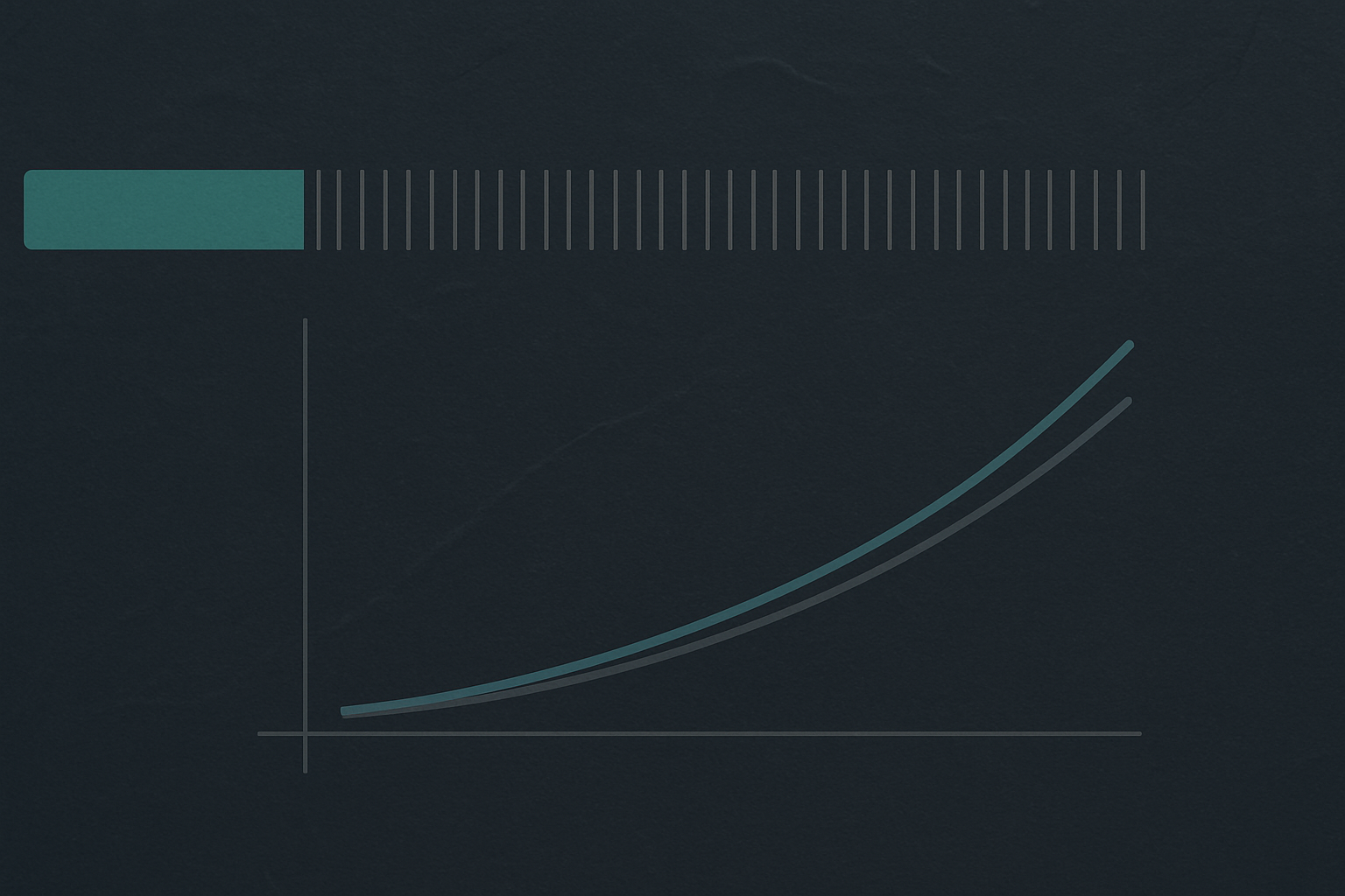
The two metrics have different bottlenecks and different optimization paths.

TTFT scales with prompt length. A 100-token prompt has tiny prefill cost. A 100,000-token prompt has substantial prefill cost. The relationship is roughly linear because prefill compute scales with the number of tokens in the prompt (more precisely, with the number of FLOPs to multiply each token through every layer). Prompt caching collapses this for cached prefixes: a request that hits a 90% prefix cache pays prefill cost only on the uncached suffix. Continuous batching can also affect TTFT positively when the scheduler can fit the prefill into a gap between other requests’ decode steps, or negatively when the prefill has to wait its turn.

TPOT scales with sequence length and inversely with available memory bandwidth. Each decode step reads the entire KV cache. As the sequence grows, the cache grows, and each step reads more bytes. TPOT therefore slowly degrades as the response gets longer, with the slope depending on the model’s per-token cache footprint. GPU choice matters: an H100 or H200 with more HBM bandwidth produces a meaningfully lower TPOT than an A100 on the same model and prompt. Quantization helps: storing the KV cache in FP8 instead of BF16 halves the bandwidth needed per step, which typically halves the TPOT growth rate.

The two metrics are in tension with throughput. The same continuous-batching mechanism that maximizes total tokens-per-second across all in-flight requests can degrade per-request TPOT when the GPU is fully saturated and one request’s decode step has to wait for others’ decode steps to share the kernel.

A contestable claim worth sitting with. Users feel TTFT and they feel TPOT. They do not feel any of the other metrics on your serving dashboard. Throughput numbers (tokens per second across the fleet, batch utilization, cost per million tokens) describe operational efficiency. They describe how the vendor’s economics work. They describe nothing about the experience of waiting for an answer and watching it type out at a comfortable speed. A serving stack that pushes throughput at the cost of TPOT is selling the customer worse latency for better unit economics, and most customers who care about the product will leave for a vendor that gets TPOT right even when it costs more per million tokens. The marketing numbers and the experience numbers are not the same numbers, and conflating them is the most common mistake in serving-stack benchmarking in 2026.

Deeper: how TTFT and TPOT combine into total response time.
Total response time is roughly TTFT + (output_token_count − 1) × TPOT. For a request that produces 500 output tokens with TTFT of 800 ms and TPOT of 40 ms, the total time is 800 + 499 × 40 ≈ 20,760 ms, about 21 seconds for a long response. The user perceives the first 800 ms as the wait and the next 20 seconds as the response materializing. Latency optimization has different implications depending on which segment you target. Cutting TTFT in half is felt immediately. Cutting TPOT in half halves the time the response takes to finish typing, which matters most on long responses. For short responses TTFT dominates; for long responses (multi-paragraph essays, code generation, reasoning-mode outputs) TPOT dominates. Most production tuning targets one or the other based on the workload mix.

The throughput-versus-latency tradeoff that continuous batching exists to manage is the central tension in serving-stack design. Bigger batches improve total tokens-per-second across the fleet and reduce per-token cost. Bigger batches also increase contention for the GPU’s per-step compute and memory bandwidth, which raises per-user TPOT. The right answer depends on what the workload values. Interactive chat workloads prioritize TPOT. Batch-inference workloads (overnight document processing, bulk classification) prioritize throughput. Hosted vendors typically run separate fleets tuned for the two cases, which is why the same model can have different latency characteristics depending on which API tier the developer is calling.

Quantization helps both metrics. FP8 weights and FP8 KV cache halve the memory traffic per step. INT4 weight quantization (GPTQ, AWQ, GGUF) further reduces weight-fetching cost. The accuracy cost is real and varies by model and quantization scheme, but for production deployments the speedup typically justifies the careful evaluation work needed to ship a quantized model.

Then: the inside is not universal

The request is done. The bytes are on the screen. The bill is committed. The trace is closed.

Six phases of the request have now been covered, and they cover everything that is universal across hosted LLM APIs. From the gateway to the streaming response, the machinery is roughly the same machine regardless of which vendor’s model is on the other end of the call.

What changes is the interior. The model inside the request is not just one shape. There are dense decoder-only transformers, sparse mixture-of-experts, recurrent state-space hybrids, and parallel diffusion language models, and the four interiors are different enough that the same prompt takes a structurally different route through the math depending on which model the gateway routed it to.

Phase 7 — The Inside Is Not Universal covers that fork in depth. The wrapper around the model is universal. The model itself is not.