Phase 4 — The Per-Token Loop

Prefill is done. The prompt’s K and V vectors sit in the cache, one set per layer per token. The LM head has produced logits for the last position. The first sampling decision is about to happen.

From here, until the model emits its stop token, the same tight loop runs over and over. One token’s worth of forward pass. One logit vector. One sampling step. One KV-cache write. Repeat. This is decode. It is memory-bandwidth-bound, not compute-bound, and that single fact is the reason all the latency optimizations in this phase exist.

One token at a time

Each iteration of the decode loop runs the same six operations.

The newest token’s ID enters the model. The embedding lookup turns it into a hidden state. Every layer runs the same arithmetic prefill ran, but on exactly one position instead of thousands: normalize, project to Q/K/V, rotate by RoPE, attend, write the new K/V to the cache, run the FFN, add residual. The attention step reads the entire KV cache up to this point. The cache contains K and V vectors for every token the model has already seen, prompt and generated. The new Q gets matched against all of them. The new K and V get appended as one new column per layer.

The final layer’s hidden state goes through the LM head. The result is a logit vector with one entry per token in the vocabulary, typically 100,000 to 200,000+ entries. The next section covers what happens to those logits before they become a sampled token. Once a token is chosen, the loop appends it to the sequence, writes its K and V into the cache, and starts again.

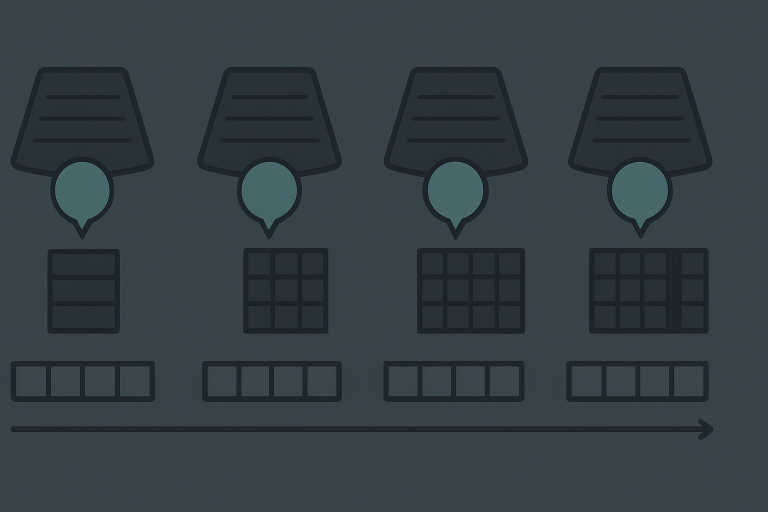
The arithmetic of one decode step is small. The single new Q vector multiplied against a few thousand cached K vectors is a handful of milliseconds of math on a modern accelerator. The expensive part is the cache read itself. Every step reads the entire cache out of HBM and feeds it through the attention units. As the sequence grows, the per-step cache-traffic cost grows linearly with it. At typical single-sequence throughput of 30 to 200 tokens per second per GPU on a frontier-scale model, the GPU’s math units are idle most of the time. They are waiting on memory.

This is what “memory-bandwidth-bound” means in practice. The GPU has a peak arithmetic throughput in the tens of TFLOPs and a peak memory bandwidth in the low TB/s. Decode operates so far below the arithmetic peak that adding more math (a draft model’s worth of extra computation, a logit-processing pipeline, a grammar-engine state machine update) costs essentially nothing. The decode loop’s tricks all exploit this asymmetry.

The logit processing pipeline

The model’s output, at every step, is a raw logit vector. Logits are unbounded real numbers, one per vocabulary entry. Before any sampling happens, the logits go through a pipeline of transformations that the developer’s API parameters control. The pipeline runs in a specific order, and the order matters because each stage depends on the one before it.

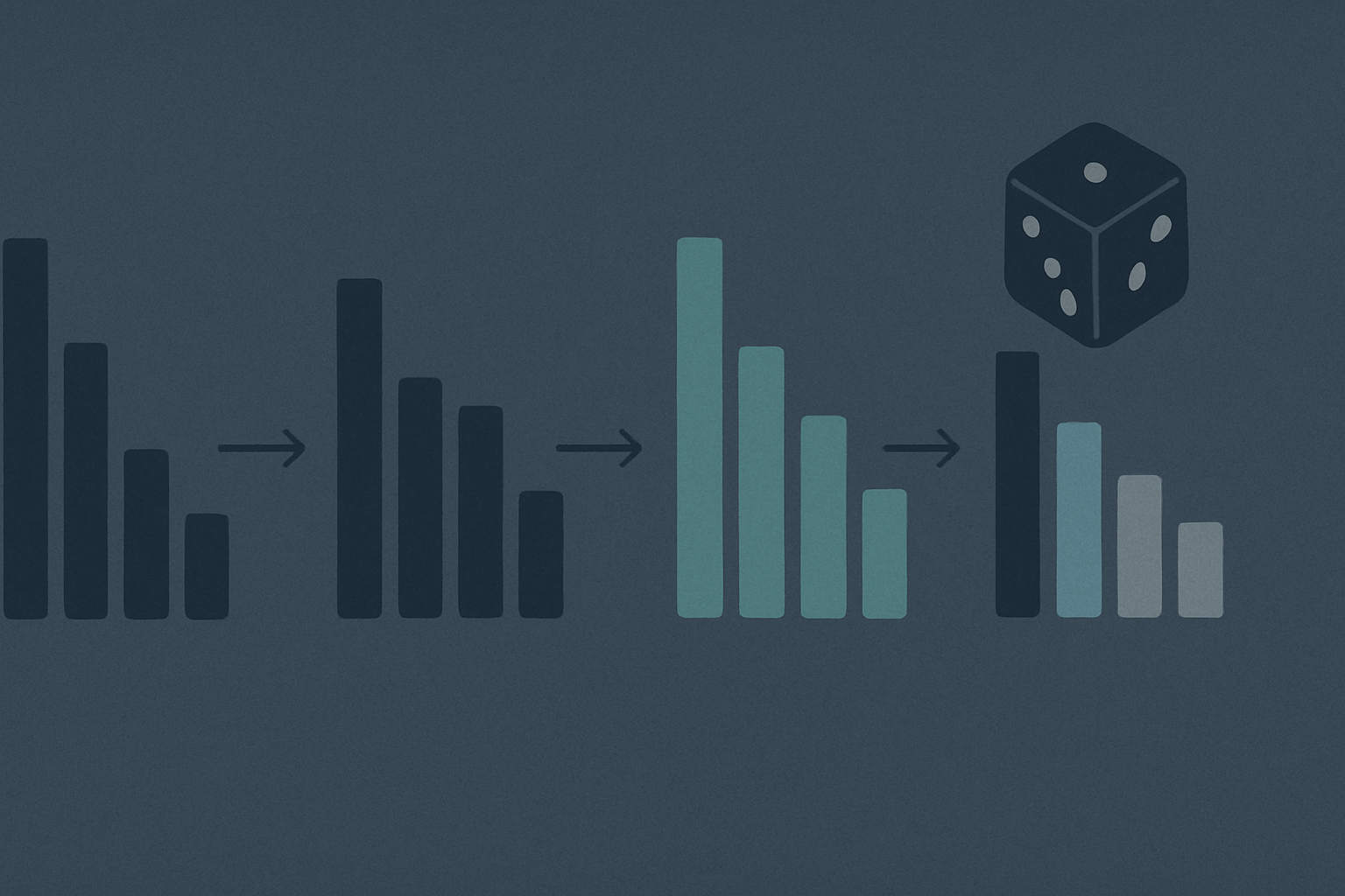
The standard pipeline, step by step.

logit_bias. A per-token additive nudge. The developer can boost or suppress specific tokens directly. Useful for narrow steering tasks (“never emit the token for the company name” or “always prefer the JSON-valid quote character”). It runs first because it is a direct modification of the raw scores.

Repetition, presence, and frequency penalties. Each subtracts a value from the logits of tokens already generated, reducing the probability of repetition. The three differ in their counting: presence is a flat per-token boolean, frequency scales with how many times the token has appeared, repetition is a multiplicative variant from the original OpenAI API. These penalties are how you push a model away from looping on its own previous output. They are also how you accidentally make a model refuse to use the word “is” twice in a paragraph if you tune them aggressively.

Temperature. The classic knob. Divide every logit by T. Lower T sharpens the distribution (the highest-probability tokens dominate); higher T flattens it (less likely tokens get more weight); T=0 collapses to greedy argmax. The relationship to perceived output is non-linear in a way that bites tuners: going from T=0.7 to T=0.8 produces a barely-noticeable shift; going from T=1.0 to T=1.2 can produce visibly degenerate output.

Top-k. Keep only the k highest-logit tokens; set all others to negative infinity. Truncates the long tail of unlikely tokens. Typical values run from 40 to a few hundred. Setting k=1 collapses to greedy.

Top-p (nucleus). After applying softmax, keep the smallest set of tokens whose cumulative probability mass exceeds p, then renormalize over that set. Truncates the tail adaptively based on confidence: when the model is confident, top-p keeps only a few tokens; when it isn’t, top-p keeps many. Values around 0.9 to 0.95 are common.

Min-p. A newer filter that sets a minimum probability threshold relative to the most likely token. If the top token has probability 0.4 and min-p is 0.1, any token with probability below 0.04 is cut. Min-p is more robust than top-p across temperatures and is increasingly the default in newer serving stacks.

Structured-output constraint masking. Optional. If the developer requested a JSON schema, regex, or grammar-constrained output, the grammar engine sets the logits of structurally invalid tokens to negative infinity. The deep dive on this is below.

Tool-call forcing. Optional. When the developer has set tool_choice to “required” or to a specific tool, the sampler can be constrained at this stage to only emit the tokens that begin a tool call (the special tokens, the tool name, the opening JSON for arguments).

Sample. The final, transformed distribution is sampled. Multinomial draw from the surviving probabilities, or argmax if temperature has collapsed to zero, or beam search if the API supports it (most don’t anymore). The seed parameter, where supported, makes this step reproducible.

Deeper: why temperature and top-p interact in counterintuitive ways.
Temperature operates on logits before softmax; top-p operates on probabilities after softmax. If you set a very low temperature (sharpening the distribution dramatically), the top one or two tokens absorb most of the probability mass, and top-p ends up retaining only those tokens regardless of the value of p. The opposite is also true: a very high temperature flattens the distribution so much that top-p retains a large fraction of the vocabulary. The two parameters are not independent, and the practical implication is that you should pick one as your primary diversity knob and leave the other near default. Most modern guides recommend tuning min-p instead, because min-p is a relative threshold that survives temperature scaling more gracefully.

The penalties and the filters all silently interact with constrained decoding in ways the average integration doesn’t notice. Apply a frequency penalty to a token that the grammar engine has decided is the only valid next token, and the sampler is sampling from a distribution where the only legal answer has been suppressed. Combined with low-temperature settings, this can produce stuck outputs where the model would have generated the right answer but the pipeline ate it. Production stacks that take structured output seriously turn off penalties when constraint masking is active.

Speculative decoding

The decode loop’s headline latency trick. Speculative decoding exploits the fact that decode is memory-bandwidth-bound to verify several tokens at once for roughly the cost of one.

A small, fast draft model runs ahead of the large target model, predicting the next several tokens (typically four to eight). The draft model is cheap enough that running it briefly costs almost nothing on the target’s wall-clock budget. The large target model then runs a single forward pass that scores all of the draft’s proposed tokens in parallel. Because each position the target evaluates costs about the same as a regular decode step (the cache read dominates either way), the target processes four-to-eight token positions for the cost of one.

A rejection-sampling rule decides which speculated tokens are kept. Tokens where the target’s distribution agrees with the draft’s are accepted. On the first disagreement, the target’s correction is used as the new token and the speculation restarts from there. The mathematical guarantee, which the whole technique stands on, is that the output distribution is identical to plain target-model sampling. There is no quality tradeoff.

The net effect is typically two-to-three times fewer sequential decode steps. On highly predictable text (boilerplate, code in a familiar style, structured output) the speedup can be larger because the draft model gets more correct guesses in a row. On unusual or unpredictable text the speedup approaches one because most drafts get rejected on the first token.

Variants worth knowing.

Medusa adds extra prediction heads to the target model itself, eliminating the need for a separate draft model. The heads are trained to predict tokens at multiple future positions in parallel.

EAGLE explores a small tree of speculations rather than a single chain, increasing the chance of finding accepted prefixes.

N-gram lookup uses a corpus-based n-gram table as the “draft model,” which is essentially free to query. Effective for repetitive structured output.

Lookahead decoding explores multiple branches in parallel and accepts the best.

Most production vendors run some form of speculative decoding in 2026, though it is not always exposed to developers as a tunable knob.

Deeper: the rejection-sampling guarantee.
The accept-reject rule for a draft token with target probability p_target(t) and draft probability p_draft(t) is: accept with probability min(1, p_target(t) / p_draft(t)). On rejection, sample from a modified distribution max(0, p_target − p_draft) normalized over the vocabulary. The proof that this produces a sample identical in distribution to vanilla target sampling is a one-page exercise in probability and is what makes speculative decoding a free win rather than a quality tradeoff. It is also why the technique cannot speed things up beyond a constant factor: the target still has to verify, and the verifier-side latency floor is the target model’s per-step cost.

Constrained decoding

The reliability technique. The grammar engine knows, at every step, which tokens would produce a structurally valid continuation of the output and which would not. Before sampling, the engine sets the logits of every structurally invalid token to negative infinity. The sampler then cannot pick an invalid token. The output literally cannot break the schema.

The mechanism is straightforward. The constraint (a JSON schema, a regular expression, a context-free grammar, or a custom format) is compiled into a state machine, typically an FSM for regex and a push-down automaton for context-free grammars. At every decode step, the engine queries the state machine: given the partial output so far, which next tokens advance to a still-valid state? The set of valid token IDs becomes a boolean mask. The mask is applied to the logits before any other sampling logic runs. Tokens marked invalid have their logit set to −∞; sampling proceeds normally over the remaining ones.

Production engines that do this well in 2026 add under 5% latency overhead per step, because the state-machine update is O(1) per token and the mask application is a vectorized operation that runs in microseconds. The main engines are Outlines (Python, the original), XGrammar (C++, optimized for speed), llama.cpp GBNF (for local inference), and the vendor “guided decoding” or “structured output” features in OpenAI, Anthropic, and Google’s APIs. The vendor-side implementations are typically a wrapper around one of the open-source engines, sometimes with proprietary optimizations.

A contestable claim worth sitting with. Structured-output enforcement is a contract, not a quality fix. The grammar engine guarantees the output parses as JSON, matches the regex, or conforms to the schema. Prompt engineering (“please respond in valid JSON, do not include any prose”) guarantees only that the output usually parses, on the kind of test inputs the developer thought to try. The gap between guarantees-it and usually-does is the gap between a stack you can build reliable systems on and a stack that produces incidents your customers find before you do. Treating structured output as a prompt-engineering thing rather than a runtime constraint is the most common reliability mistake in production LLM integrations in 2026, and it is a mistake every modern serving stack already gives you the tools to avoid.

Deeper: why compiling a JSON schema to a state machine is not trivial.
A JSON schema can be recursive (an array of objects, each containing an array of objects). The corresponding grammar is context-free, not regular, so the state machine has to be a push-down automaton with a stack tracking nesting depth. Worse, the tokenizer’s vocabulary doesn’t align with JSON syntax: the token " might be its own token in one model, part of a larger token like ": in another, and yet another in a third. Compiling the schema involves walking every token in the vocabulary against the partial-output state to figure out which tokens are legal at that point, and pre-computing as much of that work as possible. Modern engines like XGrammar do this offline during model load and cache the per-state legal-token masks aggressively. The result is constant-time lookup at decode time, which is what makes constrained decoding cheap enough to use by default.

Closing the loop

When the loop terminates, the complete assistant response is in the sequence. The conditions that end the loop are checked on every step:

• The model has emitted its end-of-sequence (EOS) token, or its model-specific stop token (Llama’s <|eot_id|>, Claude’s equivalent).
• A developer-supplied stop string has appeared in the output.
• The max_tokens limit has been reached.
• A structured-decoding state machine has reached a terminal accepting state.

The user has not seen the response yet because tokens have been streamed back as they were generated. Phase 5 — Streaming Back and Rendering covers the streaming and rendering side: incremental detokenization, the UTF-8 buffering gotcha, output-side moderation, tool-call interception, and the client-side Markdown rendering that turns the stream into formatted text in the user’s browser.

The compute-bound half built the cache. The memory-bound half drained it. Now the bytes head back.