Phase 7 — The Inside Is Not Universal

The same chat-completion endpoint. The same JSON schema. The same SSE stream. The same usage receipt at the end. Behind that universal interface, four genuinely different architectures are now in production, and the same prompt takes a structurally different route through the math depending on which of them the gateway routed it to.

Phase 1 through Phase 6 covered the wrapper. The wrapper has converged. Auth, gateway, tokenize, schedule, prefill, decode, stream, bill. Every vendor has a version, and the versions are interchangeable enough that swapping providers in production code is mostly a matter of changing a few constants and adapting the error handler.

The interior has not converged. It has fragmented. Four distinct cognitive shapes are running under the same chat-completion surface in 2026, and the differences matter for capability, cost, latency, and the engineering work required to ship them.

Dense decoder-only

This is the workhorse and the architecture everyone learned the field on. Llama, Mistral, the GPT-class models through GPT-4o, the Claude-class models, the original Gemini family.

The structure is simple and uniform. A stack of N identical transformer layers. Each layer has a multi-head attention block (or one of its modern variants: grouped-query attention, multi-query attention, multi-latent attention) followed by a fully-connected feed-forward network. The same shape, repeated, top to bottom, with residual connections threading through every layer and a final un-embedding projection that turns the last hidden state into a distribution over vocabulary tokens.

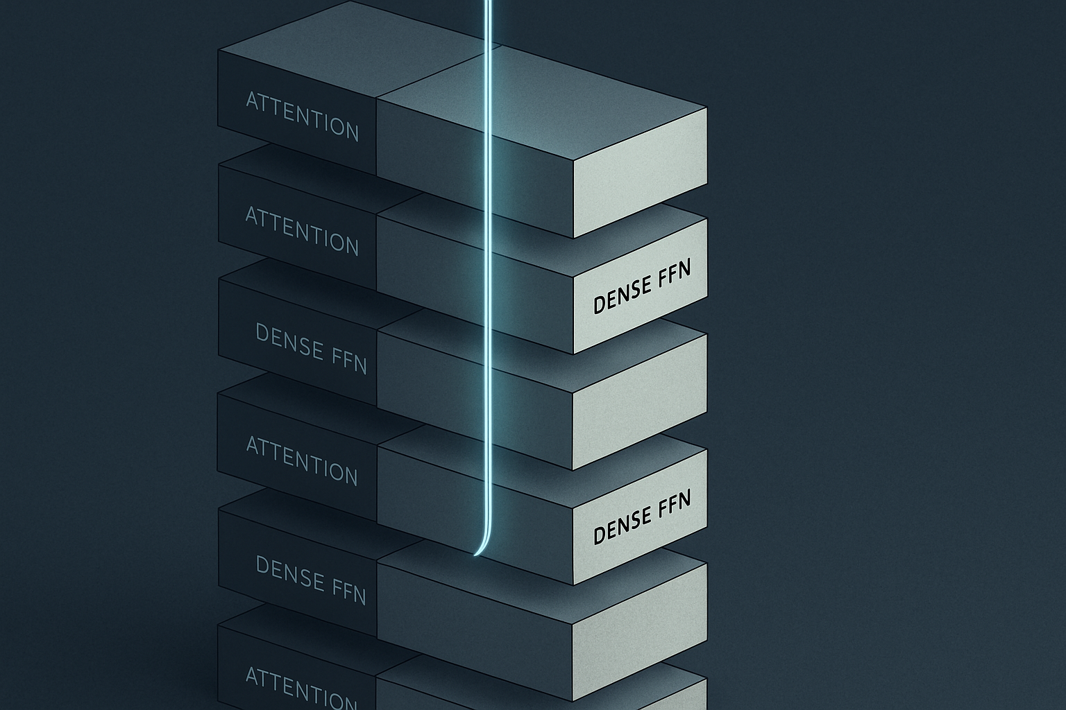
Every parameter activates on every token. A 70-billion-parameter dense model performs roughly 140 billion FLOPs of compute for every single token (two FLOPs per parameter per token, ignoring attention compute which adds a separate term scaling with sequence length squared). The relationship is direct, predictable, and brutal. Doubling the parameter count doubles the per-token compute cost. There is no clever trick that lets you scale capacity without scaling per-token inference cost on a dense model. The compute bill is the parameter count, every step, every token.

This is why dense models are getting harder to push to the frontier. Training a 1-trillion-parameter dense model is hard but doable with enough compute. Serving the resulting model at chat-product latency to millions of users is expensive enough that the unit economics collapse. The closed-weights frontier labs have stayed largely dense (with significant qualifications around what GPT-5 and Claude-class models actually look like, which the labs have not disclosed) because dense models train more stably, the pipeline is well-understood, and the labs have the compute budget to absorb the inference cost. The open-weights frontier has moved decisively to MoE for exactly the opposite reason.

What dense models give you in return for the cost is consistency. Every parameter has been touched by every training token. There are no routing decisions to go wrong at inference time. There is no expert-imbalance failure mode where a poorly-routed token gets less compute than it needed. The model is dumb, in a good way, about how it uses its capacity. It uses all of it, all the time, on everything.

Deeper: why per-token compute matters more than total parameter count.
Marketing copy talks about parameter count because the number sounds impressive. The serving stack cares about per-token activated parameter count, because that is what determines how many tokens per second a GPU can produce. A 70B dense model and a 600B MoE model with 30B active parameters per token cost roughly the same to serve per token. The MoE model has more capacity for knowledge and skills, sure, but the relevant inference economics number is “activated per token,” not “total.” Every benchmark that reports parameter count without distinguishing the two is misleading.

Mixture-of-experts

Mixtral was the first to push the architecture into mainstream production in 2023. Through 2024 and 2025 the architecture ate a remarkable fraction of the open-weights frontier. Mixtral, DeepSeek-V2, DeepSeek-V3, Qwen-MoE, Grok, the various Llama-MoE variants, Snowflake Arctic. The pattern is now standard enough that any new open-weights frontier release that isn’t MoE is the surprising one.

The mechanic. Inside each transformer layer, the feed-forward network is replaced by a router and N expert FFNs (each expert is itself a feed-forward network the same shape as a dense FFN would have been). For every token, the router computes a small dot-product score against each expert, picks the top-k experts (typically top-1 or top-2), routes the token to those experts, runs the FFN computation, and combines the results with a weighted sum. The other N-k experts do nothing for that token. Their parameters live on the GPU but no compute touches them.

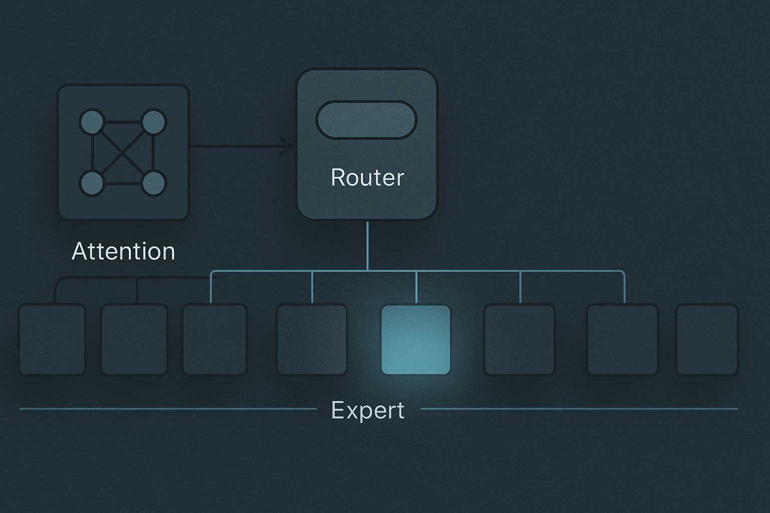
DeepSeek-V3 is the cleanest worked example for late-2025 / early-2026. The model has roughly 671 billion total parameters and activates roughly 37 billion per token, for a sparsity ratio of about 18:1. Each transformer layer has 256 routed experts plus 1 shared expert (the shared expert is a small FFN that always activates on every token, capturing common features that don’t benefit from routing). The router picks 8 of the 256 routed experts per token. Add the shared expert and the token sees compute equivalent to 9 expert FFNs out of 257, which works out to the 37B-active figure.

That 18:1 ratio is the central trick. The model has 671B parameters worth of knowledge capacity and 37B parameters worth of per-token inference cost. The per-token compute cost is similar to a dense 37B model. The knowledge capacity is similar to a dense 671B model (with caveats: routing makes some skills harder to learn, some experts get more training signal than others, and the cross-expert coordination has to be learned). For workloads where the bottleneck is knowledge coverage rather than per-token reasoning depth, the tradeoff is dramatically favorable.

Three things make MoE inference engineering nontrivial.

Load balancing. A naively trained router converges to using a small fraction of the experts heavily and ignoring the rest. Training-time auxiliary losses (load-balancing loss, importance loss) explicitly penalize uneven routing to keep the experts from collapsing into a few hot ones. At inference time, batches arrive with the routing already baked in by the trained router, and skew across experts in a batch translates directly into idle GPU capacity on under-utilized expert devices.

Expert capacity per batch. A single batch might want to route 500 tokens to expert 42 and 50 tokens to expert 17. If expert 42’s per-batch capacity is 256, some of those 500 tokens get dropped or rerouted. The capacity factor is a knob the serving stack tunes against the training-time setting, and getting it wrong silently degrades quality.

Expert parallelism and all-to-all communication. Models like DeepSeek-V3 are too large to fit on a single GPU, so the experts get sharded across many devices. Routing a token to its assigned experts requires sending the token’s hidden state across the interconnect to whichever device holds the right expert, running the FFN, and gathering results back. This all-to-all communication is one of the dominant costs in serving large MoE models on multi-node clusters, and it is one of the main reasons NVLink-class interconnect bandwidth matters as much as raw GPU compute for MoE-heavy fleets.

A contestable claim worth sitting with. MoE has not won the open-weights race because it is a better architecture in some abstract sense. MoE has won because it lets a research lab with limited training compute push frontier capability at a per-query inference cost the lab can actually afford to serve. The closed-weights labs with the largest compute budgets are keeping dense (or are very secretive about whatever hybrids they are running) because dense pipelines train more stably and the engineering surface is smaller. The result is that “MoE is open-weights, dense is closed-weights” is becoming a structural feature of the frontier in 2026, not a momentary accident, and that split is widening rather than collapsing.

State-space and hybrid

Attention is O(n²) in sequence length for the attention computation itself, and the KV cache it produces grows linearly with sequence length and gets read on every decode step. Both of those costs are real and both of them get worse as context windows push past 100k tokens.

State-space models replace attention (sometimes entirely, sometimes in a fraction of the layers) with a recurrent scan over a fixed-size hidden state. The recurrence updates the state at each token position. Crucially, the state shape does not grow with sequence length. There is no growing KV cache to read on every decode step. There is just the state, the same size always, being updated in place.

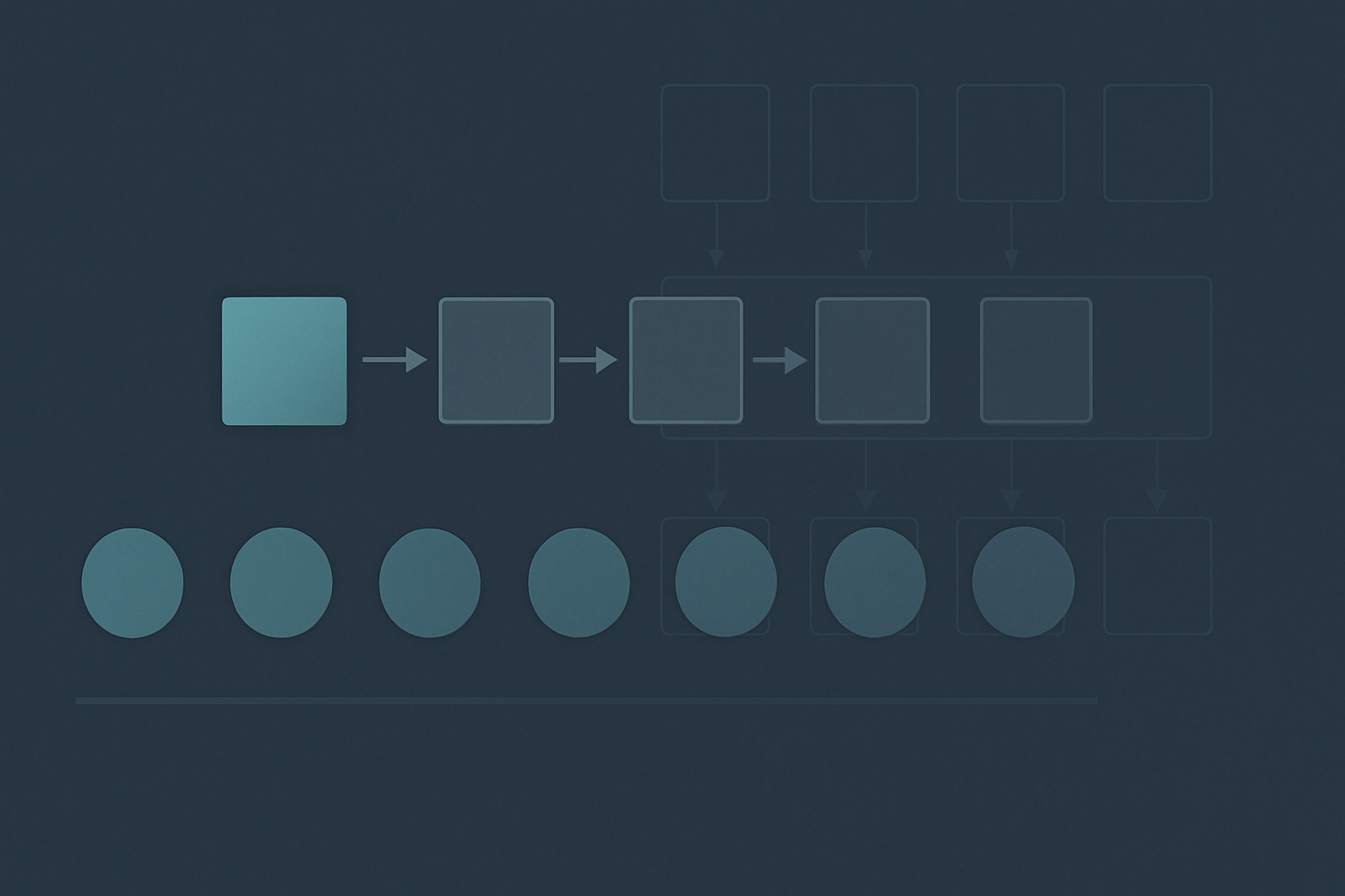
Mamba (Albert Gu and Tri Dao, 2023) was the first selective state-space architecture that was competitive with transformers on language modeling at small-to-medium scales. The selective part is the important part. Earlier SSMs (S4, S5) had a fixed transition matrix that did not depend on the input, which limited their ability to do content-dependent reasoning. Mamba’s transition matrix depends on the current token’s embedding, which lets the model decide what to remember and what to forget based on what it just saw. This is, very loosely, how the architecture recovers something attention-like in a recurrent form.

Pure-SSM models have had a harder time matching transformer quality at the largest scales, which is why most production systems that use SSMs use hybrids. Jamba (AI21, 2024) interleaves Mamba layers with transformer layers and adds MoE on top. Falcon-H1 (TII, 2025) uses a Mamba+transformer interleaving designed to keep most of the long-context cost in the Mamba layers while keeping a small number of attention layers for the content-routing tasks SSMs are weaker at. Zamba (Zyphra, 2024) uses a similar hybrid pattern with shared attention blocks.

Serving implications.

The KV cache problem changes shape. On a pure-SSM layer there is no KV cache at all, just a fixed-size state. On a hybrid model with some attention layers, the attention layers still need a cache, but the cache is proportional to the fraction of layers that are attention layers, not to the full model depth. A 64-layer hybrid where 8 layers are attention has roughly 1/8 the KV cache memory pressure of a 64-layer transformer at the same context length. For long-context workloads (document analysis, code-base reasoning, long agent traces), this is a material cost win.

Decode latency at long context changes shape. A transformer’s decode step reads the entire KV cache from HBM, which means decode TPOT degrades as the context grows. An SSM’s decode step reads only the fixed-size state from HBM, so TPOT does not degrade with context length on SSM layers. Hybrids inherit a mix of both behaviors.

The tradeoffs the architecture pays for these wins are real. The compressed fixed-size state cannot represent every possible long-range dependency a growing KV cache could. Tasks that require retrieving a specific token from far back in the context (needle-in-a-haystack benchmarks) are harder for SSMs than for transformers. Hybrids partially recover this capability by including some attention layers. The current evidence (as of mid-2026) is that well-designed hybrids match or beat transformer quality on most benchmarks at long context while paying meaningfully less serving cost, but the picture is still evolving fast.

Diffusion language models

Generation is not autoregressive on these models at all. There is no per-token loop. Phase 4, the per-token decode loop, does not happen.

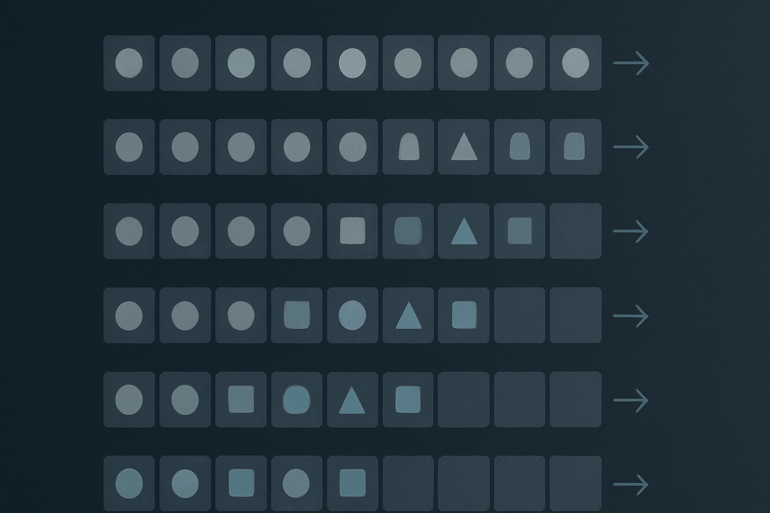
The model starts from a fully-masked sequence (every position is a placeholder token) and predicts all positions in parallel using bidirectional attention (no causal mask, because every position can attend to every other position). The most-confident predictions are committed. The rest are re-masked. The model runs again. Predictions are committed and remasked. The process repeats for some number of denoising steps, with the number of steps decoupled from the length of the sequence being generated.

The architecture has been talked about as a research curiosity for years (D3PM, MaskGIT, SUNDAE, the various continuous-diffusion attempts) but only recently became commercially viable for language. Mercury (Inception Labs, 2025) was the first commercial diffusion LM with claimed throughput in the 1000-tokens-per-second range. LLaDA (Renmin University / Ant Group, 2025) is the most-cited open research model. Gemini Diffusion (Google, late 2025) is the highest-profile production deployment, available in preview as of early 2026.

The shape of the speed/quality tradeoff is completely different from autoregressive serving.

On an autoregressive model, generating a 1000-token response requires 1000 sequential decode steps, each of which has to wait for the previous one to finish. Latency is fundamentally bounded by the number of output tokens times the per-step time. There is no way to parallelize across the output sequence.

On a diffusion LM, generating a 1000-token response requires N denoising steps, where N is configurable. Each denoising step processes all 1000 positions in parallel. A 16-step diffusion generation runs in roughly 1/60 of the steps a 1000-token autoregressive generation would, although each diffusion step does substantially more work per step than a single autoregressive decode step. The end result on current hardware is generation throughput that can be several times faster than the best autoregressive serving on the same model size, at the cost of quality that is still somewhat behind frontier autoregressive models for the same parameter count.

For applications where total generation latency matters more than per-token quality (real-time conversational agents, code completion, IDE inline suggestions, voice-mode pipelines), diffusion LMs are starting to look genuinely attractive. For applications where the marginal token quality matters most (complex reasoning, code review, long-form synthesis), autoregressive models still have the edge as of mid-2026.

The serving stack for a diffusion LM looks different enough that most of Phase 4’s discussion does not apply. There is no per-token sampling pipeline. There is no speculative decoding (the architecture is already parallel). The KV cache concept does not transfer cleanly because attention is bidirectional and the entire sequence is recomputed at every denoising step. Streaming is different too. Some diffusion-LM serving stacks stream partial committed tokens as they become confident, which gives the user a “fuzzy” experience where some tokens appear before others in non-left-to-right order. Other stacks just wait for all denoising steps to complete and emit the whole response at once.

The orthogonal axes

Two more architectural patterns are worth naming, but they compose with all four of the above rather than competing with them.

Long-reasoning models. The o-series (OpenAI), DeepSeek-R1, Claude with extended thinking enabled, Gemini with thinking enabled. These models run a long internal chain-of-thought, often thousands of tokens, before producing the visible answer. The reasoning tokens are billed as output tokens but routed to a separate channel so the developer can show or hide them. The underlying architecture can be dense, MoE, or hybrid. Long-reasoning is a training-and-inference recipe, not an architecture. It is mostly the same forward-pass machinery with a different stopping criterion and a different inference-time compute budget.

Multimodal and any-to-any. GPT-4o, Gemini, the Claude vision models, Qwen-VL, the various open-weights vision-language models. These models add an encoder front-end (vision transformer, audio spectrogram encoder, sometimes both) that produces embedding tokens which get prepended to the LLM’s input. Inside the LLM itself, the architecture is whatever the LLM is (dense, MoE, hybrid, in principle diffusion). The multimodal capability is a feature of the input pipeline, not of the language-model interior. Output modalities work the other way: tokens get emitted as usual, then a small decoder turns them back into pixels or audio.

Both of these axes can be combined with any of the four interior architectures. A multimodal long-reasoning MoE model is a plausible 2027 configuration, and pieces of it already exist in production.

What the family adds up to

Seven phases. The first six describe a wrapper that is roughly the same machine at every hosted LLM vendor. Auth, gateway, tokenize, schedule, prefill, per-token loop, stream, tool loop, terminate, bill. Phase 7 describes the four genuinely different interiors that now sit inside that universal wrapper, with two orthogonal axes that compose with all four.

The practical takeaway for anyone building product on top of LLMs in 2026. Code against the wrapper. The wrapper is stable and the conventions are converging. Treat the interior as a swappable detail, because the interior is going to keep churning yearly while the wrapper conventions ossify on a multi-year timescale. The chat-completion endpoint, the SSE stream, the four-class usage receipt, the tool-calling format, the prompt cache, the streaming gotchas. These will look approximately the same in 2028. The specific model serving on the other end will not.

The practical takeaway for anyone working on the serving stack. The interior diversity is going to keep pushing on every assumption the wrapper was built around. KV caches that don’t exist on SSM layers. Parallel denoising that doesn’t fit the per-token-loop abstraction. Routing-dependent compute distribution that doesn’t fit the batch-scheduler abstraction. Hidden reasoning tokens that the billing model has to account for separately. Every one of these has already required wrapper changes at the larger hosted vendors. More are coming.

The practical takeaway for anyone trying to predict where the field goes. The convergence is happening at one layer and the divergence is happening at another, and that is exactly the dynamic that produces a healthy ecosystem. The wrapper convergence makes products portable across vendors and architectures. The interior divergence keeps the frontier moving. The two have decoupled enough that they can now evolve on independent timescales, which is a structural improvement over the period in 2023 when the entire field had to coordinate on every change to the underlying architecture.

That coordination cost is gone. What replaces it is a serving stack that has to be polyglot about what is on the other end of its calls, and that polyglotism is the through-line of everything Phase 1 through Phase 6 actually described.

The seven phases are done. The walk is over. The model on the other end of your next API call is still doing the same nine things it was doing when you started reading. You now know roughly what each of them is.

Adjacent material on this site

• Inference (hub) — the front door to the seven-phase family. Start there to navigate back to any phase.
• Artificial Intelligence — the broader category these pages live under.