Phase 3 — Scheduling and Prefill

The request is fully prepared. Its prompt is a sequence of integers. Its attention mask is built. Its multimodal vectors are projected and inserted. It is sitting in a scheduler queue. The next two things that happen are the only two things in the whole pipeline that are genuinely the model’s work.

The scheduler picks the batch the request will run in. The model runs prefill: one big parallel forward pass through every layer, computing K and V vectors for every token in the prompt and storing them in a cache for the decode loop that follows. Prefill is the compute-bound half of a request. It is also where the most consequential serving optimizations in 2026 live.

How the scheduler packs the batch

A GPU running an LLM is at its most efficient when it is doing the same operation across many tokens in parallel. The serving runtime’s job is to keep the GPU saturated by packing requests together. The way it does this has changed dramatically since 2023.

The wrong way is static batching. You wait for some fixed number of requests to arrive, you start them as a batch, you wait for all of them to finish, and then you process the next batch. The slowest request in the batch sets the throughput for everyone in it. Short prompts wait for long prompts. Decoded outputs wait for the request with the most tokens to emit. GPU utilization is wasted in the idle gaps. This is how serving worked in the first wave of LLM products and it was painfully inefficient.

The right way is continuous batching, sometimes called in-flight batching. Requests join the batch and leave the batch on every single step. A request can be admitted mid-batch as soon as another request finishes. A finished request returns its GPU slot to the pool immediately. The batch is a sliding window of in-flight work, not a fixed group that drains together. This is the single biggest throughput improvement in modern LLM serving and is the default in vLLM, SGLang, TensorRT-LLM, and every hosted vendor’s stack.

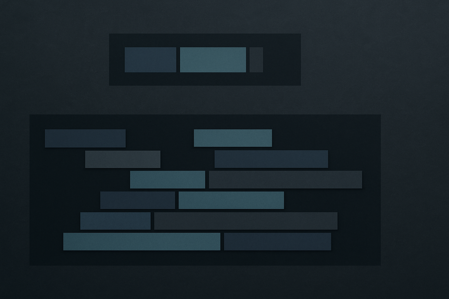
Chunked prefill is the second optimization. A long prompt (say 50,000 tokens) takes a substantial fraction of a second to prefill end to end. If you naively schedule it as one operation, it stalls every other request that wanted to run a decode step on the same GPU during that window. This is head-of-line blocking. Chunked prefill splits a long prompt into chunks (typically 512 or 1,024 tokens) so the prefill interleaves with other requests’ decode steps. The long-prompt request still takes the same total time, but no other request has to wait for it.

Prefix and radix caching are the third optimization. If many requests share a system prompt, or a common tool schema, or a long conversation history that the user is iterating against, the K and V vectors for that shared prefix are identical across requests. Computing them once and reusing them for every subsequent request with the same prefix skips most of the prefill work for that prefix. vLLM calls this Automatic Prefix Caching. SGLang implements it as RadixAttention, which uses a radix tree to identify the longest shared prefix across in-flight requests. Hosted providers expose it either explicitly (Anthropic’s cache_control markers) or automatically (OpenAI’s prompt caching). The hit rate on production traffic with stable system prompts and tool schemas is routinely above 80%. The economic effect is large: a cached prefix turns most of the prefill cost into a pointer lookup.

KV-cache allocation decides how the cache memory gets carved up across in-flight requests. The naive approach reserves one large contiguous block per request, sized to its expected total length. That wastes memory in two directions: short requests reserve more than they need, and the cache memory fragments as requests come and go. The breakthrough was PagedAttention (the vLLM paper, 2023), which treats the KV cache as virtual memory. The cache is split into fixed-size blocks (typically 16 or 32 tokens of K and V per layer). Each request gets a per-layer block table mapping logical positions in its sequence to physical block IDs. Blocks are allocated on demand as the sequence grows. The block table is the indirection layer that lets the runtime pack many sequences into the same pool without contiguous-block waste.

Prefill/decode disaggregation is the most recent optimization, and the one not every stack runs yet. Prefill and decode have different bottlenecks. Prefill is compute-bound: the math units are working full-tilt on a large parallel operation. Decode is memory-bandwidth-bound: the math units are mostly waiting on the cache. Running them on the same GPU means one of those strengths is wasted at any given moment. Some serving stacks (DistServe, Mooncake, certain vendor deployments) run prefill on one GPU pool and decode on another, transferring the KV cache between them at the handoff. The KV-transfer cost is real but smaller than the throughput gain when the prefill-to-decode ratio is right.

Deeper: the PagedAttention block-table indirection in one paragraph.
Imagine the KV cache as a large pool of fixed-size blocks, each block holding the K and V for some small fixed number of token positions (16 or 32) for one layer. Each sequence has a per-layer block table: a small array of block IDs in the order the sequence reads them. When the sequence grows by 16 tokens, the runtime allocates one more block from the pool and appends its ID to the block table. Attention reads tokens by walking the block table and gathering K and V from the physical blocks the table points to. The indirection means physical blocks for one sequence are not necessarily contiguous, which is exactly what enables the pool to absorb arbitrary mixes of long and short sequences without fragmentation. It also enables copy-on-write sharing of identical prefix blocks across requests, which is what makes prefix caching actually cheap to implement.

By the time the scheduler is done, the request is in a batch, its KV cache has block allocations, its prefix-cache hits (if any) have been noted, and it is ready to consume GPU cycles. Prefill begins.

The KV cache, in detail

The KV cache is the central memory constraint in LLM serving. Understanding why requires understanding what prefill is actually computing.

In a decoder-only transformer, generating token t requires the model to attend over every token at positions 0 through t−1. Attention is a function of Query, Key, and Value vectors. The Q for the current token is computed from its own hidden state. The K and V for every prior token were computed when those tokens were originally processed. If the model had to recompute K and V for every prior token at every step, generating n tokens would scale like O(n²) work per step. For a thousand-token output, that’s roughly a million times more compute than necessary.

The KV cache fixes this by storing the K and V vectors as they are computed and reading them back on subsequent steps. The first time a token is processed (during prefill, or as it is decoded), the model computes K and V from its hidden state and writes them to a per-layer cache. Every subsequent step that needs to attend to that position reads the cached K and V back. Each decode step’s attention cost becomes O(n) (read the cache, attend, sample) instead of O(n²) (recompute everything).

The cost is memory. The cache grows linearly with sequence length and linearly with batch size, and the per-token footprint is decided by the model architecture. The rough formula:

KV bytes ≈ 2 × n_layers × n_kv_heads × head_dim × seq_len × batch × bytes_per_value

The 2 is one K plus one V. For a Llama-class 70B model running in BF16, with 80 layers, 8 KV heads (because Grouped-Query Attention is the default), 128 head dimensions, two bytes per value, that comes out to about 320 KB per token in the cache. A 2,048-token context costs about 650 MB per sequence. Batch size 32 takes about 21 GB. None of that includes the model weights themselves, which take another 140 GB on a 70B model in BF16. Even with weights sharded across multiple GPUs, the cache is a substantial share of total HBM footprint.

This is why decode is memory-bandwidth-bound. Each decode step reads the entire cache out of HBM to compute attention scores against the new Q vector. The math operation itself is cheap. The cache shuffling is what the GPU spends its time on.

Four optimizations matter, in roughly the order most serving stacks adopt them.

Grouped-Query Attention (GQA) and Multi-Query Attention (MQA). The model has more query heads than KV heads, and multiple query heads share one K/V pair. Llama-3-70B has 64 query heads and 8 KV heads, so the cache is 8x smaller than it would be with full Multi-Head Attention. The quality loss versus full MHA is small. The memory savings are not. Almost every frontier-scale model trained since 2024 uses GQA.

PagedAttention. Already covered above. The headline number is that PagedAttention typically recovers 30–60% of HBM that was previously wasted to fragmentation.

KV-cache quantization. Storing K and V in FP8 or INT8 instead of BF16 halves or quarters the memory footprint. The quality loss is small for K and V because attention is somewhat tolerant of noise in those vectors. Quantizing the cache lets the same GPU hold more concurrent sequences.

Prefix caching. Reusing the K and V for a shared prefix across requests. Already covered.

Deeper: why bigger context windows make this worse, not just longer.
A model that supports a 1M-token context window does not just need more cache per request. It needs the cache architecture to scale gracefully. The naive approach of allocating one big contiguous block per sequence becomes catastrophic at million-token contexts: you cannot pack many concurrent 1M-token sequences on a single accelerator’s HBM at all. PagedAttention’s block-table indirection is what makes long contexts even feasible in production, because it lets the runtime allocate blocks on demand and reclaim them aggressively as sequences finish. The headline-friendly “we support 2M tokens” claims of 2026 models are downstream of paged-cache machinery that did not exist three years earlier.

A contestable claim worth sitting with. The single most important architectural decision in serving frontier LLMs in 2026 is not the size of the model or the choice of attention kernel. It is whether you let the KV cache fragment your GPU memory. PagedAttention’s contribution was treating the cache as virtual memory. Every modern serving stack now does it because the alternative wastes between a third and two thirds of HBM to fragmentation, and HBM is the binding cost of running these models in production.

Inside one transformer layer

With the KV cache machinery understood, the per-layer prefill operation is comprehensible.

A modern decoder-only transformer has somewhere between 28 and 100+ identical layers stacked. Each layer is a function that takes the previous layer’s output (the hidden state, a tensor of shape [batch, seq_len, hidden_dim]) and returns a new tensor of the same shape. The model’s first operation is an embedding lookup that turns the input token IDs into the first hidden state. The model’s last operation is the LM head, which projects the final hidden state into a vocabulary-sized vector of logits. Between those two ends, every layer does the same thing.

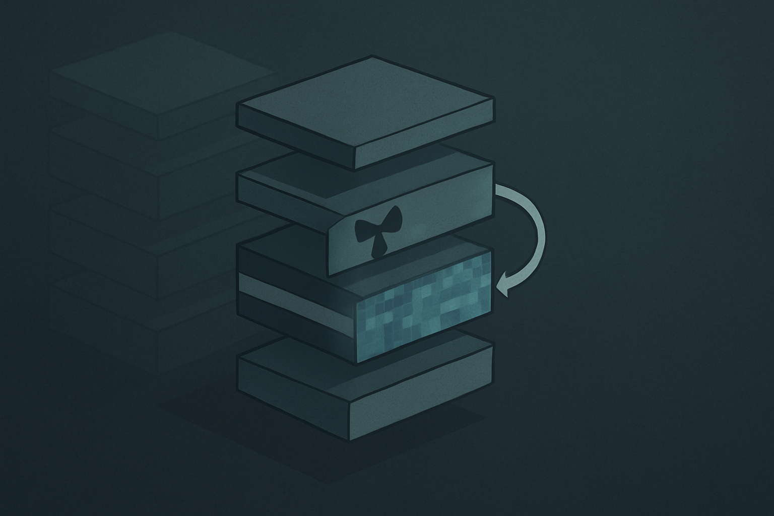
Inside one layer, in order:

Input normalization. RMSNorm in most modern models, sometimes LayerNorm in older designs. Normalization stabilizes training and inference by keeping activation magnitudes bounded. Modern models put the norm before each sub-block (“pre-norm”) rather than after, because pre-norm trains more reliably at large depths.

QKV projection. The hidden state is multiplied by a learned weight matrix to produce Query, Key, and Value vectors per attention head. In a model with N query heads and K KV heads (with GQA, N ≠ K), this is one matrix multiply that produces all of them. The Q, K, V vectors are then reshaped to separate the heads.

Positional encoding. RoPE rotates Q and K by an angle proportional to the token’s position. This is the most common positional encoding in 2026 frontier models, and it has its own deep-dive section below. Position is not added to the hidden state at the model’s input; it is applied inside attention, per layer, on Q and K only.

Attention. softmax(Q · Kᵀ / √dₖ) · V, with the causal mask blocking the upper triangle so each token can only attend backward. This is the operation that mixes information across positions. Multi-head means this happens in parallel across many heads, each learning different patterns. With GQA, query heads share KV heads. Computed in practice with a fused kernel (FlashAttention or its successors) that never materializes the full attention matrix.

Write to the KV cache. The K and V for every position in this prefill step get written to the per-layer cache, so the decode loop can read them back without recomputation.

Output projection. The attention output is multiplied by another learned matrix to bring it back to the hidden dimension. A residual connection adds the layer’s input to the output of attention, which is what lets gradient flow through many layers without vanishing.

Post-attention normalization. Another norm before the feed-forward sub-block.

Feed-forward network. This is where the family of model architectures diverges. In a dense decoder-only model, the FFN is two or three linear projections with a non-linearity in the middle (SwiGLU is the default in modern frontier dense models, replacing GELU and ReLU from earlier generations). In a mixture-of-experts model, the FFN is replaced by a router and many expert FFNs, with only a few experts activating per token. In a state-space model layer, the FFN slot is occupied by a recurrent scan. Phase 7 covers the architectural fork in depth. Here it is enough to say that per-layer compute is roughly equally split between attention and FFN in dense models, with FFN dominating somewhat in narrow-and-deep architectures.

Residual add. The FFN output is added to its input via another residual connection.

After every layer has been applied, the model applies a final normalization to the hidden state and then projects it through the LM head (the “unembedding” matrix) to produce logits over the vocabulary. During prefill, only the last position’s logits are needed for the first output token. The rest of the work is purely to fill the KV cache with K and V vectors for the decode loop to read.

RoPE: how position gets injected

Attention by itself is order-blind. The dot product Q · Kᵀ does not depend on where in the sequence Q and K originated. If you shuffled a sentence and ran it through pure attention, the model would produce the same output as on the unshuffled sentence. This is a problem because language is sequential. Position has to come from somewhere.

Older transformer designs added a learned positional embedding to the input hidden state, one row of the embedding table per position. This worked but had two weaknesses. The model could not generalize beyond the maximum position seen in training, because positions past that point had no learned embedding. Position information also decayed through the layer stack, because the residual stream was the only carrier of positional signal and it got mixed with content at every layer.

Rotary Position Embedding (RoPE) replaced this. Position is not added to the hidden state at the input. Instead, the Q and K vectors are rotated by an angle proportional to the token’s position, applied inside each attention block, at every layer. Because attention computes Q · Kᵀ, and rotating both Q and K by their respective angles affects the dot product by the difference of the angles, the rotation injects information about the relative distance between two tokens rather than the absolute position of either.

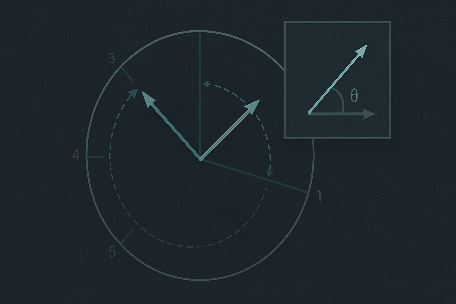
This has three consequences worth pulling out.

Position information is per-layer, not just at the input. Every layer’s attention sees the same positional rotation applied to its own Q and K. The signal doesn’t have to survive a long residual chain.

The model attends to relative distance. A token at position 100 attending to a token at position 50 sees the same effective angular relationship as a token at position 200 attending to a token at position 150. This is what makes models trained with RoPE generalize better to longer sequences than their training distribution.

Context-length extension becomes tractable. Techniques like NTK-aware scaling, YaRN, and Position Interpolation modify the RoPE angle formula to make a model trained on, say, 8k tokens behave reasonably at 32k or 128k. None of these gives you something for free, but the existence of RoPE makes the extension possible at all. Pre-RoPE models could not be extended this way.

Deeper: the rotation formula in one paragraph.
RoPE pairs up the dimensions of Q (or K) into 2D pairs, and rotates each pair in its own plane by an angle that scales with the token’s position and inversely with a frequency that varies across dimensions. Lower-dimension pairs rotate fast (high frequency: they encode short-range structure), higher-dimension pairs rotate slow (low frequency: they encode long-range structure). The dot product between a rotated Q at position p and a rotated K at position q ends up depending on the difference p − q, with each pair contributing at its own frequency. This is the mechanism by which a single attention operation can be made aware of both local and long-range positional relationships simultaneously.

Attention, the operation

The core operation, per head, is:

Attention(Q, K, V) = softmax( (Q · Kᵀ) / √dₖ ) · V

Read step by step.

Q · Kᵀ produces a matrix of scores. The entry at row i, column j is the dot product of Query i with Key j, which measures how much token i should attend to token j. Larger means more relevant.

Divide by √dₖ keeps the scores’ magnitudes from blowing up as the head dimension grows. Without this, the softmax that follows would saturate, and gradients (during training) or attention distributions (during inference) would degenerate.

The causal mask sets entries above the diagonal to negative infinity, so that token i cannot attend to any token at position j > i. This is what makes the model autoregressive. Without the mask, a token could “see the future” and the model couldn’t generate left to right.

Softmax turns the score matrix into a probability distribution per row. Each row sums to one. The values represent how much weight token i puts on each previous token’s value vector.

Multiply by V produces a weighted sum of value vectors, per row. That’s the attention output: each token’s new representation is a learned mixture of every prior token’s V vector, weighted by the relevance scores.

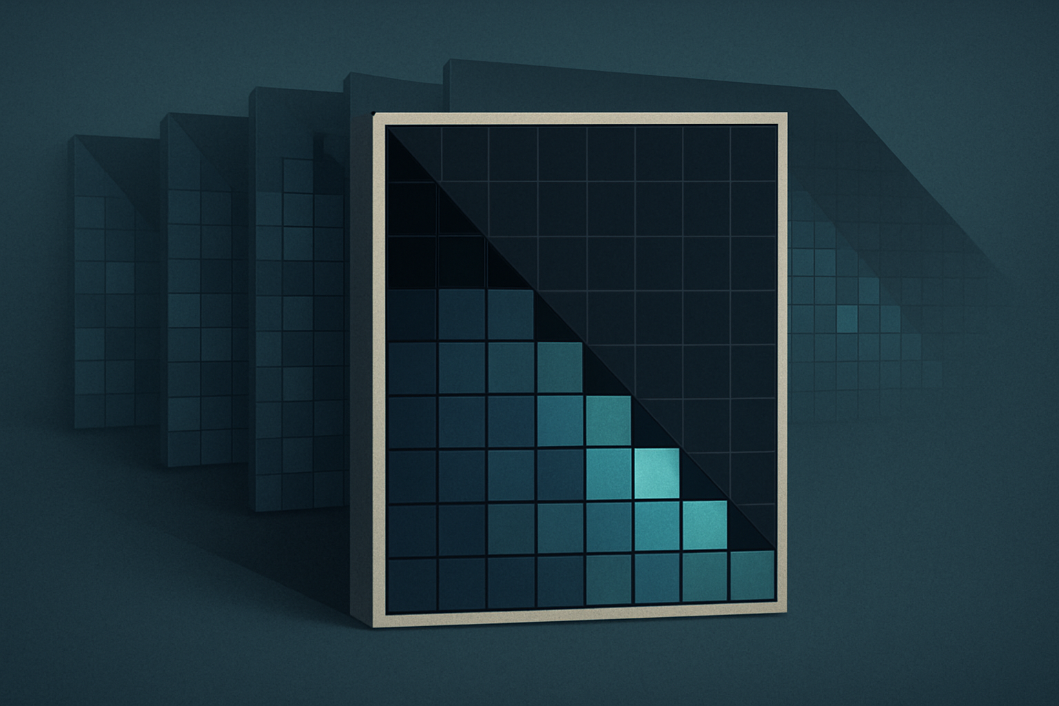
Multi-head attention runs this in parallel across many heads, each with its own learned Q, K, V projections. Heads specialize during training. Some heads track syntactic relationships. Some track long-range topic coherence. Some track coreference (who does “he” refer to). Some learn patterns that are not legible to humans but consistently contribute. The outputs of all heads are concatenated and projected back to the hidden dimension.

The biggest practical concern is memory. The full attention matrix is seq_len × seq_len, which for a 32k-token prompt is a billion entries per head, far too large to materialize in HBM. The fix is FlashAttention (and its successors FlashAttention-2 and FlashAttention-3), a tiling trick that computes attention block by block without ever holding the full matrix in slow memory. The block of Q rows being processed at any moment fits in fast on-chip memory; the corresponding blocks of K and V are streamed in. The math is identical to standard attention; the memory access pattern is the breakthrough. FlashAttention is what makes long contexts even computable on modern GPUs.

Deeper: why FlashAttention matters more than the model architecture for long contexts.
The headline complaint about transformer attention is that it’s O(n²) in sequence length, both in compute and in memory. FlashAttention does not change the compute side; it still does O(n²) math. What it changes is the memory access pattern. By tiling the attention computation so the intermediate softmax statistics fit in fast on-chip memory, FlashAttention turns attention from “O(n²) memory traffic” into “O(n) memory traffic.” The asymptotic compute cost is unchanged but the realized throughput on a GPU goes up by an order of magnitude or more on long sequences, because for those sequences memory bandwidth was the binding constraint, not arithmetic. This is also why much of the “we made attention sub-quadratic” research direction (linear attention, kernel methods, locality-sensitive variants) has not displaced standard attention in frontier models: standard attention plus FlashAttention is fast enough in practice that the theoretical advantage of sub-quadratic methods rarely pays for itself given their quality cost.

The compute-bound half

By the time prefill finishes, every prompt token has flowed through every layer. Every layer’s K and V vectors for every prompt token are sitting in the KV cache. The last position’s logits are in hand, ready for the first sampling decision.

This is the compute-bound half of the request, and it is where most of the GPU’s arithmetic for the whole request happens. A 4,000-token prompt followed by a 200-token completion does more math during prefill than during the entire decode loop, even though decode runs many more sequential steps. The decode loop is memory-bound and reads what prefill computed.

Phase 4 — The Per-Token Loop covers what happens next: the single-token forward pass, the logit processing pipeline, sampling, and speculative decoding. The wrapper around the model is done. The interior is what’s left.